
This post and the full series has been elaborated jointly with Ana Isabel Prieto, Sergio Villanueva and Luis Búrdalo.
In the previous article we commented on the difficulty faced by Threat Hunting analysts as a result of the high number of domains registered daily by an organization. This makes it difficult to analyze and locate potentially malicious domains, which may go unnoticed among so much traffic. For this reason, in an attempt to facilitate the analyst’s task, the use of alternative techniques based on Machine Learning is proposed. Before presenting the different tests performed, the article introduces the algorithms to be used for the detection of anomalies in the domains.
To begin with, it is necessary to comment that having a large and varied database is fundamental for a model to be able to detect potentially malicious domains reliably, since its parameters are going to be adjusted in an environment that must be similar to the real one.
However, there is great difficulty in identifying patterns in high-dimensional data, and even more difficulty in representing such data graphically and expressing them in a way that highlights their similarities and differences. This is where the need arises to use a powerful data analysis tool such as PCA (Principal Components Analysis).
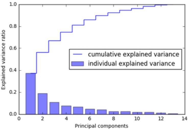
The main objective of PCA is to transform a large set of variables into a smaller one that contains most of the original information. To do this, new dummy variables (principal components) are created in the directions of maximum variance from the linear combination of the original variables, so that each principal component contains the weights of each of the original characteristics. In addition, these new variables are not correlated among themselves, and are calculated according to the amount of variability they explain, so that the first principal component is the one that explains the most variability in the original data.
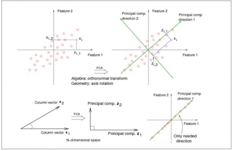
Moreover, since each of the principal components is a linear combination of the original variables, this allows us to know which original variables are more important in each principal component and, therefore, to identify which variable or variables have contributed to the fact that, for example, a certain domain is different from the rest [2].
To reduce the dimensionality of the problem, a PCA is applied to the original database of domains with their extracted lexical features, in order to extract as many principal components (PC) as necessary to explain 95% of the variability of the data. These new variables are then used by the unsupervised classification models to label each domain as “normal” or “anomalous”.
The unsupervised algorithms chosen in this case for the detection of anomalous domains have been two: Isolation Forest and One-Class SVM.
Isolation Forest
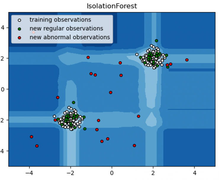
The first of the algorithms considered in this study is Isolation Forest [3]. This algorithm would fall within the family of decision trees, since it combines the performance of a set of “if-else” classifiers. By means of random cuts on the variables of the dataset, these classifiers isolate the different observations of the dataset, assigning to each one the average number of cuts necessary for its total isolation. Isolation Forest is based on the premise that those observations with more peculiar characteristics will be isolated more quickly from the rest of the data, thus requiring fewer partitions for their isolation [3].
One Class SVM
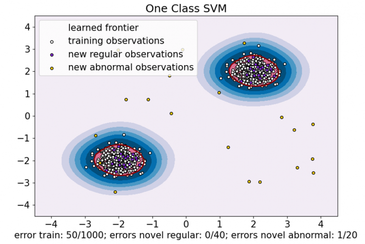
The second algorithm considered in this study is One Class SVM [5]. It is an extension of the classical support vector machines for the case of unlabeled data. Here, instead of separating two classes by means of a hyperplane in the feature space, what is attempted is to frame the data sample within a minimum volume hypersphere, so that the outermost points that are left out are considered outliers [5].
What is considered anomalous?
It is important to note that these algorithms classify as anomalous those elements that are significantly different from the rest, which is not always because they are malicious. For example, if the activity of different users within an organization were monitored, the behavior of system administrators might appear to be anomalous simply because they perform specific tasks that are very different from those of other employees.
On the other hand, it should also not be assumed that malicious activity is significantly less frequent than lawful activity. For example, in the case of a DoS attack, malicious activity would be much greater than lawful activity, so the algorithms used in this series of articles may not be able to detect such activity.
In the next post we will present the tests and results obtained by applying the algorithms already discussed, as well as some details about the database we have worked with.
References
- [1] scikit-learn: Data Compression via Dimensionality Reduction I – Principal component analysis (PCA) – 2020. (2020). bogotobogo. https://www.bogotobogo.com/python/scikit-learn/scikit_machine_learning_Data_Compresssion_via_Dimensionality_Reduction_1_Principal_component_analysis%20_PCA.php
- [2] Shalizi, C. (2013). Advanced data analysis from an elementary point of view. Cambridge: Cambridge University Press.
- [3] Liu, F. T., Ting, K. M., & Zhou, Z. H. (2008, December). Isolation forest. In 2008 eighth ieee international conference on data mining (pp. 413-422). IEEE. (https://cs.nju.edu.cn/zhouzh/zhouzh.files/publication/icdm08b.pdf)
- [4] IsolationForest example. (2022). Retrieved 4 April 2022, from https://scikit-learn.org/stable/auto_examples/ensemble/plot_isolation_forest.html#sphx-glr-auto-examples-ensemble-plot-isolation-forest-py
- [5] Schölkopf, B., Williamson, R. C., Smola, A., Shawe-Taylor, J., & Platt, J. (1999). Support vector method for novelty detection. Advances in neural information processing systems, 12. (https://papers.nips.cc/paper/1999/file/8725fb777f25776ffa9076e44fcfd776-Paper.pdf)
- [6] One-Class SVM versus One-Class SVM using Stochastic Gradient Descent. (2022). Retrieved 4 April 2022, from https://scikit-learn.org/stable/auto_examples/linear_model/plot_sgdocsvm_vs_ocsvm.html#sphx-glr-auto-examples-linear-model-plot-sgdocsvm-vs-ocsvm-py